TL;DR:
Data preparation is 60–80% of every ML project — and the #1 reason models succeed or fail.
- Garbage in = garbage out → even the best models fail with bad data
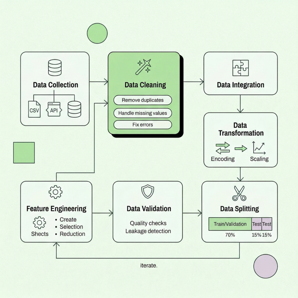
- The process includes 7 core steps: collect → clean → integrate → transform → engineer → validate → split
- Feature engineering is often the biggest driver of model performance
- The most common killer: data leakage (models “cheating” with future info)
- Other pitfalls: poor splitting, class imbalance, bad missing-data handling, no EDA
- Best practice: use end-to-end pipelines to avoid errors and ensure reproducibility
- In 2026, AI agents automate 50–70% of data prep — but fundamentals still matter
Here’s a stat that hasn’t budged much over the years: data practitioners still spend somewhere between 60% and 80% of their project time on data preparation. Not modeling. Not tuning hyperparameters. Not deploying. Just getting the data ready.
Your model is only as smart as the data behind it.
That ratio makes sense when you think about it. A well-tuned algorithm fed messy, inconsistent, or leaky data will confidently produce wrong answers. Garbage in, garbage out, as the old saying goes. The truth is, data preparation isn’t the unglamorous warm-up act before the “real” ML work begins. It is the work. Or at least, the most consequential part of it.
The good news? You don’t have to do it all by hand anymore. AI agents, automated feature engineering, and platforms like Pecan’s Predictive AI Agent are reshaping the workflow from end to end. But automation works best when you understand the fundamentals underneath it. That’s what this guide is for.
Whether you’re a marketing ops manager building your first churn model, a RevOps lead scoring pipeline architect, or a BI analyst tired of the spreadsheet swivel-chair, we’ll walk you through the full data prep lifecycle: the seven core steps, production-ready code examples (Python and SQL), the ten pitfalls that tank most projects, and a ready-made checklist you can keep at your desk.
Let’s dig in.
What is data preparation for machine learning?
Data preparation (sometimes called data preprocessing or data wrangling) is the process of transforming raw, real-world data into a clean, structured format that machine learning algorithms can actually learn from. Think of it as the bridge between “we have tons of data” and “we have a working predictive model.”
It covers a broad sweep of activities: collecting data from multiple sources, cleaning up missing values and inconsistencies, integrating datasets that don’t share a common schema, engineering features that capture real business signals, validating that nothing has leaked across your training boundary, and splitting the data so your model gets an honest evaluation.
The reason it dominates project timelines isn’t a failure of planning. It’s that real business data is messy by nature. Customer records live in Salesforce, transaction histories sit in a data warehouse, marketing engagement data comes from HubSpot, and none of them agree on what “customer_id” means. Reconciling all that is genuinely hard work.
If you’re curious about the broader context of how machine learning fits into predictive analytics, that’s a great companion read. But right now, let’s focus on the prep work that makes those models possible.
Why data preparation makes or breaks your models
You’ve probably heard variations of this claim, but it bears repeating: an estimated 85% of AI initiatives fail, and poor data quality is consistently cited as a leading cause. That number has become something of a cliché in the industry, sure. But the underlying reality hasn’t changed.
ML algorithms are pattern-matching engines. They’ll find patterns whether or not those patterns are real. Feed a model training data that contains future information it shouldn’t have access to (a problem called data leakage), and it’ll happily learn to “predict” outcomes it already knows the answer to. Your validation metrics will look phenomenal. Then you deploy, and everything collapses.
One well-documented Kaggle competition saw a model’s AUC score plummet from 0.99 to 0.59 after data leakage was discovered. A research review found at least 294 published papers affected by the same issue. These aren’t edge cases.
Well-prepared data does several things at once: it reduces noise so real signals come through, it prevents the model from memorizing artifacts instead of learning patterns, it ensures your evaluation metrics reflect real-world performance, and it makes the model’s outputs trustworthy enough to actually act on.
For teams working on use cases like churn prediction or customer lifetime value modeling, the stakes are especially high. A churn model built on leaky data might tell you to “save” customers who were never leaving. A LTV model trained on inconsistent transaction records could wildly misallocate your retention budget. The prep work matters.
the 7-step data preparation workflow
Step 1: Data collection
Every ML project starts with a question: “What do we want to predict?” and, immediately after, “What data do we have that might help?”
Data typically comes from multiple sources: your CRM (Salesforce, HubSpot), transactional databases, marketing automation platforms, third-party APIs, spreadsheets (yes, still), and increasingly, cloud data warehouses like Snowflake or BigQuery. The challenge isn’t usually getting some data. It’s getting the right data, from the right time window, in a format you can work with.
Start with exploratory data analysis (EDA). Even before you clean anything, get a feel for what you’re working with.
Python: Initial data exploration
import pandas as pd

df = pd.read_csv('customer_data.csv')

# Quick overview

print(df.shape)          # How many rows and columns?

print(df.dtypes)         # What data types are we dealing with?

print(df.isnull().sum()) # Where are the gaps?

print(df.describe())     # Statistical summary

# Check for duplicates

print(f'Duplicate rows: {df.duplicated().sum()}')
SQL: Data extraction with basic cleaning built in
SELECT

    customer_id,

    UPPER(TRIM(city)) AS city,

    CAST(signup_date AS DATE) AS signup_date,

    COALESCE(age, AVG(age) OVER()) AS age

FROM customers

WHERE signup_date >= '2024-01-01'

  AND age BETWEEN 18 AND 100;
A small tip: resist the temptation to grab every column you can find. Start with what you believe will be predictive, then expand. Too many irrelevant columns create noise, slow down training, and can even introduce leakage if you’re not careful.
Step 2: Data cleaning
This is where you roll up your sleeves. Real-world data is messy. Missing values, duplicate entries, inconsistent formatting, typos, outliers that might be errors or might be genuinely extreme observations. Cleaning is the process of identifying and resolving all of it.
Handling missing values
There’s no one-size-fits-all solution here. Mean or median imputation works for continuous features when data is missing randomly. Forward-fill is useful for time-series. Sometimes the best move is to drop rows entirely, but only if you have enough data and the missingness is truly random.
One often-overlooked insight: the fact that a value is missing can itself be informative. If 30% of customers never filled in their income field, that non-response might correlate with behavior. Consider creating a binary “is_missing” indicator alongside your imputation.
Python: Missing value handling
from sklearn.impute import SimpleImputer

# Median imputation (robust to outliers)

imputer = SimpleImputer(strategy='median')

df[['age', 'income']] = imputer.fit_transform(

    df[['age', 'income']]

)

# Create missingness indicator before imputing

df['income_missing'] = df['income'].isnull().astype(int)

# Forward-fill for time series data

df['daily_revenue'] = df['daily_revenue'].ffill()
Removing outliers
Outliers deserve careful thought. A customer who spent $50,000 in a single transaction might be a data error, or might be your best customer. Domain knowledge matters here. Statistical methods like Z-score (flag anything beyond 3 standard deviations) or IQR-based filtering are good starting points, but always inspect what you’re removing.
Python: Outlier detection with IQR
Q1 = df['purchase_amount'].quantile(0.25)

Q3 = df['purchase_amount'].quantile(0.75)

IQR = Q3 - Q1

lower = Q1 - 1.5 * IQR

upper = Q3 + 1.5 * IQR

# Filter or flag (flagging is often safer)

df['is_outlier'] = (

    (df['purchase_amount'] < lower) |

    (df['purchase_amount'] > upper)

).astype(int)
For more on keeping your data honest, the Pecan team wrote a solid piece on data validation methods that actually work.
Step 3: Data integration
Most predictive models need data from more than one source. You’ll join customer demographics with transaction histories, layer in marketing engagement data, maybe pull in external signals like seasonality or macroeconomic indicators.
This step sounds simple (it’s just a JOIN, right?) but it introduces a surprising number of issues. Key mismatches between systems, different granularity levels (daily vs. monthly), conflicting definitions (is “revenue” gross or net?), and duplicate records that multiply when you merge.
SQL: Building a unified customer feature set
SELECT

    c.customer_id,

    c.age,

    c.region,

    t.total_spend,

    t.avg_order_value,

    t.purchase_count,

    t.days_since_last_purchase,

    e.email_open_rate,

    e.total_clicks

FROM customers c

LEFT JOIN (

    SELECT

        customer_id,

        SUM(amount) AS total_spend,

        AVG(amount) AS avg_order_value,

        COUNT(*) AS purchase_count,

        DATEDIFF(day, MAX(purchase_date),

            GETDATE()) AS days_since_last_purchase

    FROM transactions

    GROUP BY customer_id

) t ON c.customer_id = t.customer_id

LEFT JOIN (

    SELECT

        customer_id,

        AVG(opened::int) AS email_open_rate,

        SUM(clicks) AS total_clicks

    FROM email_engagement

    GROUP BY customer_id

) e ON c.customer_id = e.customer_id;
If your organization struggles with nested or hierarchical data structures, data flattening is a technique worth learning. It transforms complex multi-level datasets into the flat, tabular format that ML algorithms expect.
Step 4: Data transformation
Raw features often aren’t in a format that algorithms can use directly. Transformation covers two main tasks: encoding categorical variables into numeric representations, and scaling numeric features so they play nicely together.
Encoding categorical variables
For categories without a natural order (colors, regions, product types), one-hot encoding is the standard approach. For ordinal categories (“low,” “medium,” “high”), label encoding preserves the ordering. Target encoding can be powerful for high-cardinality categories but requires careful cross-validation to avoid leakage.
Python: Encoding examples
import pandas as pd

from sklearn.preprocessing import LabelEncoder

# One-hot encoding (most common)

df = pd.get_dummies(

    df, columns=['region', 'product_type']

)

# Label encoding for ordinal features

le = LabelEncoder()

df['tier_encoded'] = le.fit_transform(df['tier'])

SQL: One-hot encoding at the query level

SELECT

    customer_id,

    CASE WHEN plan = 'Basic'

         THEN 1 ELSE 0 END AS is_basic,

    CASE WHEN plan = 'Premium'

         THEN 1 ELSE 0 END AS is_premium,

    CASE WHEN plan = 'Enterprise'

         THEN 1 ELSE 0 END AS is_enterprise

FROM subscriptions;
Feature scaling
Features on different scales (age: 0 to 100, income: 0 to 1,000,000) cause problems for distance-based algorithms (KNN, SVM) and gradient-based optimizers. Two popular approaches:
- Min-Max normalization rescales everything to a 0 to 1 range. Good when you know the bounds.
- Standardization (Z-score) centers data around mean = 0, standard deviation = 1. More robust to outliers and generally the safer default.
Python: Scaling within a pipeline (the right way)
from sklearn.preprocessing import StandardScaler

from sklearn.model_selection import train_test_split

X_train, X_test, y_train, y_test = train_test_split(

    X, y, test_size=0.2, random_state=42

)

# IMPORTANT: fit on train, transform both

scaler = StandardScaler()

X_train_scaled = scaler.fit_transform(X_train)

X_test_scaled = scaler.transform(X_test)  # no fit!
That last point deserves emphasis. Fit your scaler on the training set only, then use it to transform the test set. Fitting on the full dataset before splitting is one of the most common forms of data leakage.
Step 5: Feature engineering
Feature engineering is where domain expertise meets data science, and it’s often the single biggest lever for improving model performance. The goal is to create new features that capture business-relevant patterns your raw columns don’t express directly.
Python: Creating business-relevant features
import pandas as pd

# Time-based features

df['account_age_days'] = (

    pd.Timestamp.now() -

    pd.to_datetime(df['signup_date'])

).dt.days

# Behavioral ratios

df['purchase_frequency'] = (

    df['total_purchases'] / df['account_age_days']

)

df['avg_order_value'] = (

    df['total_spend'] / df['total_purchases']

)

# Recency feature (days since last activity)

df['days_inactive'] = (

    pd.Timestamp.now() -

    pd.to_datetime(df['last_purchase_date'])

).dt.days

SQL: Window functions for temporal features

SELECT

    customer_id,

    purchase_date,

    amount,

    LAG(amount) OVER (

        PARTITION BY customer_id

        ORDER BY purchase_date

    ) AS prev_purchase_amount,

    AVG(amount) OVER (

        PARTITION BY customer_id

        ORDER BY purchase_date

        ROWS BETWEEN 6 PRECEDING AND CURRENT ROW

    ) AS rolling_7_avg,

    ROW_NUMBER() OVER (

        PARTITION BY customer_id

        ORDER BY purchase_date

    ) AS purchase_sequence_num

FROM transactions;
If you’re managing a lot of features, dimensionality reduction (PCA, feature selection via mutual information or permutation importance) can help keep things manageable. But don’t reach for it prematurely. Sometimes the best path is simply automated feature engineering, which can generate hundreds of candidate features from your raw data and let the algorithm sort out which ones matter.
Step 6: Data validation and quality checks
This step gets skipped more often than it should, and it’s usually where catastrophic errors hide. Before you split and train, validate your prepared dataset.
Key checks to run:
- Data leakage audit: For every feature, ask: “Would I actually have this information at prediction time?” If a feature is suspiciously predictive, investigate. A “customer_status” column that encodes whether someone already churned is an obvious example, but leakage is often subtler.
- Distribution sanity check: Plot your features. Look for unexpected spikes, bimodal distributions, or values that shouldn’t exist (negative ages, future dates).
- Class balance check: If your target variable is imbalanced (e.g., 2% churn rate), you’ll need to account for that in splitting and training. We’ll cover this in the pitfalls section.
- Correlation check: Highly correlated features add noise without information. Drop or combine them.
- Data type verification: Ensure numeric columns are actually numeric, dates are parsed correctly, and categorical columns don’t have unexpected cardinality.
Step 7: Data splitting
The final step: divide your prepared data into training, validation, and test sets. The standard split is roughly 70/15/15 or 80/10/10, depending on dataset size.
Python: Stratified train/test split
from sklearn.model_selection import train_test_split

X = df.drop(columns=['churned'])

y = df['churned']

# Stratify to maintain class distribution

X_train, X_test, y_train, y_test = train_test_split(

    X, y,

    test_size=0.2,

    random_state=42,

    stratify=y  # critical for imbalanced targets

)
For time-series use cases like demand forecasting, never randomize. Always split chronologically: train on the past, validate on the near future, test on the further future. Random shuffling would leak future information into training and give you unrealistically good metrics.
Putting it all together: a production-ready pipeline
In practice, you don’t want to run these steps as a loose collection of scripts. Scikit-learn’s Pipeline and ColumnTransformer let you bundle preprocessing and modeling into a single reproducible object that prevents leakage by design.
Python: End-to-end sklearn pipeline
from sklearn.pipeline import Pipeline

from sklearn.compose import ColumnTransformer

from sklearn.preprocessing import (

    StandardScaler, OneHotEncoder

)

from sklearn.impute import SimpleImputer

from sklearn.ensemble import (

    RandomForestClassifier

)

numeric_features = [

    'age', 'income', 'purchase_amount',

    'days_inactive'

]

categorical_features = ['region', 'plan_type']

numeric_transformer = Pipeline(steps=[

    ('imputer', SimpleImputer(strategy='median')),

    ('scaler', StandardScaler())

])

categorical_transformer = Pipeline(steps=[

    ('imputer', SimpleImputer(

        strategy='most_frequent')),

    ('encoder', OneHotEncoder(

        handle_unknown='ignore'))

])

preprocessor = ColumnTransformer(

    transformers=[

        ('num', numeric_transformer,

            numeric_features),

        ('cat', categorical_transformer,

            categorical_features)

    ]

)

model = Pipeline(steps=[

    ('preprocessor', preprocessor),

    ('classifier', RandomForestClassifier(

        random_state=42,

        class_weight='balanced'

    ))

])

# Fit on training data, predict on test

model.fit(X_train, y_train)

accuracy = model.score(X_test, y_test)

print(f'Test accuracy: {accuracy:.3f}')
The beauty of this approach: all transformations (imputation, scaling, encoding) are fitted only on training data and automatically applied to test data during prediction. No accidental leakage.
The 10 pitfalls that derail ml projects
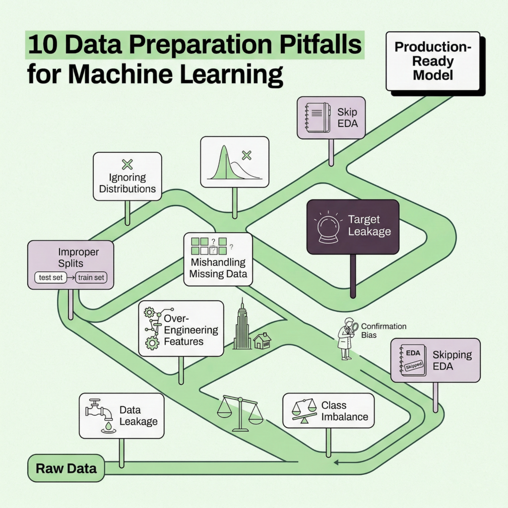
1. Data leakage (the silent killer)
Leakage occurs when information from outside the training window sneaks into your model. It produces spectacular validation results and catastrophic production failures. Three common forms: target leakage (features derived from the outcome you’re predicting), train-test contamination (fitting transformations on the full dataset), and temporal leakage (using future data to predict the past). Always ask: “Would I have this feature at the moment I need to make this prediction?”
2. Ignoring class imbalance
If 2% of your customers churn, a model that predicts “no churn” for everyone achieves 98% accuracy. Wonderful, and also completely useless. Use stratified splitting, consider SMOTE or class_weight=’balanced’, and evaluate with F1-score or AUC-ROC instead of raw accuracy.
3. Improper train/test splitting
Evaluating on training data, randomly splitting time-series, or peeking at the test set during development. Each of these inflates your perceived performance. Once you look at the test set, it stops being a test set.
4. Ignoring data distributions
Anscombe’s quartet is a famous demonstration: four datasets with identical summary statistics but wildly different shapes. Always visualize. Always. Plot histograms, box plots, scatter matrices. Skewed distributions may need log transforms; bimodal ones might indicate mixed populations.
5. Over-engineering features
More features is not always better. After a certain point, you hit the curse of dimensionality. Highly correlated features introduce multicollinearity. Features that look predictive in training might not generalize. Start lean, add deliberately, and validate each addition.
6. Mishandling missing data
Dropping every row with any missing value can eliminate a huge chunk of your dataset. Imputing with statistics from the entire dataset (including test data) introduces leakage. Not distinguishing between data that’s missing randomly versus systematically can bias your model. Be thoughtful about which strategy fits each column.
7. Scale differences between features
A feature ranging from 0 to 1,000,000 will dominate a feature ranging from 0 to 1 in any distance-based or gradient-based algorithm. Scale your features. And remember: fit the scaler on training data only.
8. Survivorship bias in data collection
If you only train on customers who stuck around long enough to generate data, you’re implicitly filtering out the very population you’re trying to predict (early churners). Make sure your dataset represents the full spectrum of outcomes.
9. Confirmation bias in feature selection
Selecting features because they “should” matter based on intuition, rather than letting the data speak. Or worse, cherry-picking features that happen to boost metrics on this particular dataset. Use systematic selection methods: mutual information, permutation importance, SHAP values.
10. Skipping exploratory data analysis
Jumping straight to modeling without understanding the data is the root cause of most other pitfalls on this list. Take the time to look at your data. Seriously. A 30-minute EDA session can save weeks of debugging.
How ai agents are transforming data prep in 2026
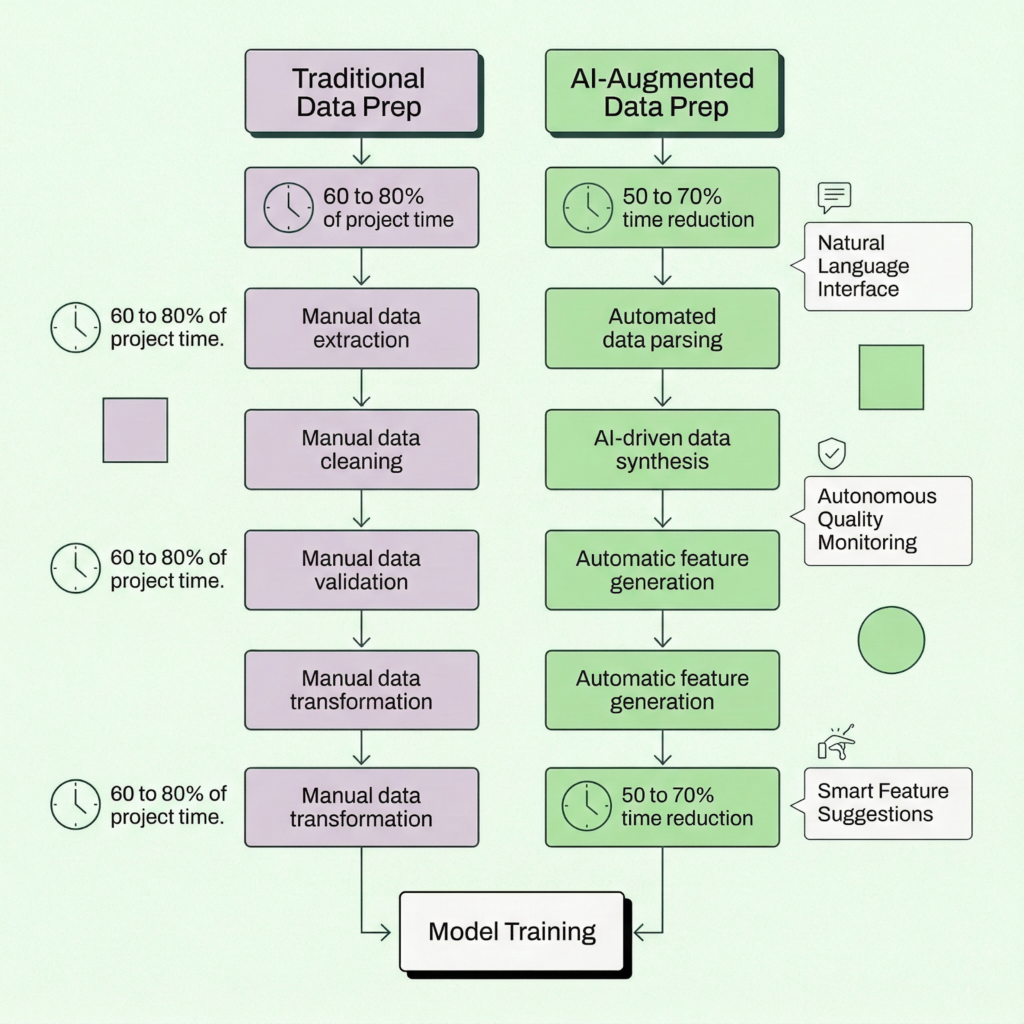
Data preparation has been the bottleneck of ML work for as long as ML work has existed. But 2025 and 2026 have seen a genuine shift, driven by AI agents that can understand, clean, and transform data with minimal human direction.
The landscape is moving fast. Google Cloud introduced Data Engineering and Data Science agents for BigQuery and Colab Enterprise, letting teams describe business intent in natural language and receive automated pipelines. Prophecy launched its v4 platform with AI agents that generate visual data prep workflows from plain-English descriptions. ThoughtSpot added agentic data preparation to its Analyst Studio. And across the board, companies report 50% to 70% reductions in analysis time after adopting AI-assisted data prep.
What these tools share is a common pattern: you describe what you want in business language, the agent handles the technical translation, and a human reviews the output. The agents aren’t replacing data engineers. They’re amplifying them. As one industry analyst put it, these tools act as force multipliers, not replacements.
For teams exploring automated predictive analytics for the first time, this shift is a huge deal. You no longer need a dedicated data science team to go from raw data to working predictions. But, and this is worth stressing, you still need to understand the fundamentals. Automation makes the process faster. It doesn’t make poor data decisions less costly.
How Pecan automates data preparation
Pecan’s approach to data prep is a bit different from the general-purpose tools we just mentioned. Instead of giving you a blank canvas with AI suggestions, Pecan’s Predictive AI Agent handles the full predictive workflow end to end: from your raw data to validated, production-ready predictions. Data preparation is embedded in the pipeline, not a separate chore you tackle before the “real work” begins.
Here’s what that looks like in practice:
Automated feature engineering
Pecan’s engine analyzes your data structure and automatically generates features tailored to each column type. Continuous variables get statistical aggregations (averages, standard deviations, min/max, linear-fit coefficients from historical trends). Categorical variables are encoded using context-appropriate methods: one-hot, ordinal, or target encoding. Date columns are decomposed into day-of-week, month, seasonality patterns, and relative time distances. Behind the scenes, the platform also applies advanced techniques like denoising autoencoders and clustering for lookalike identification.
Intelligent feature selection
Not all features earn their spot. Pecan uses permutation importance tests and SHAP values to identify which features genuinely contribute to predictive power, and drops the rest. This happens automatically, but the results are transparent: you can see exactly which features the model relies on and why.
Built-in guardrails
The platform includes automatic data leakage detection, overfitting checks, and class imbalance handling. These aren’t optional add-ons; they’re baked into every model build. For teams without deep ML expertise, this safety net is critical.
Natural language interface
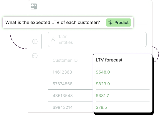
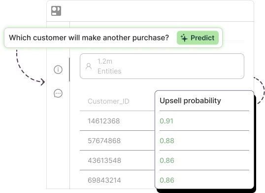
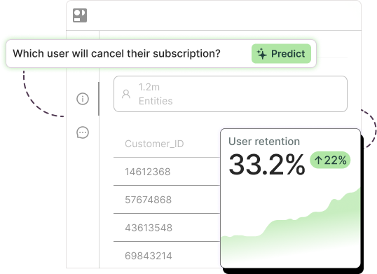
With Pecan’s Predictive Chat, you start by asking a business question in plain English: “Which customers are most likely to churn in the next 90 days?” or “What will demand look like for product X next quarter?” The agent interprets your question, maps it to the appropriate predictive workflow, and guides you through refining the setup. No SQL required (though Pecan’s Predictive Notebook supports SQL for teams that prefer it).
Direct integration where decisions happen
Predictions don’t live in a dashboard you check once a week. They flow directly into your existing tools: Salesforce, HubSpot, Snowflake, BigQuery, Redshift, Databricks. Each prediction comes with confidence scores and explanations, so your team can act with context.
For a deeper look at how Pecan’s automated data science works under the hood, including the modeling techniques (Bayesian optimization, LightGBM, CatBoost, LSTM, Prophet) and validation methodology, check out Pecan’s Data Science: A Peek Behind the Scenes.
And if you’re evaluating multiple ML platforms, the team put together a candid guide on evaluating machine learning companies (including Pecan itself) that’s worth a read.
Your data preparation checklist
Keep this handy. Whether you’re doing this manually or using an automated platform, every ML project should pass through these checks.
| Phase | Checkpoint | Status |
| Collect | Business question clearly defined | ☐ |
| Collect | All relevant data sources identified and accessible | ☐ |
| Collect | EDA completed (shape, types, distributions, missing %) | ☐ |
| Clean | Missing values handled (with strategy documented) | ☐ |
| Clean | Duplicates removed | ☐ |
| Clean | Outliers investigated (kept, removed, or flagged) | ☐ |
| Clean | Formats standardized (dates, text casing, units) | ☐ |
| Integrate | Datasets joined correctly (no fan-out or lost records) | ☐ |
| Integrate | Key definitions aligned across sources | ☐ |
| Transform | Categorical features encoded appropriately | ☐ |
| Transform | Numeric features scaled (fit on train only) | ☐ |
| Engineer | Domain-relevant features created | ☐ |
| Engineer | Feature importance evaluated | ☐ |
| Engineer | Redundant/correlated features removed | ☐ |
| Validate | Data leakage audit passed (no future info in features) | ☐ |
| Validate | Class balance checked and addressed | ☐ |
| Validate | Distributions visually inspected | ☐ |
| Validate | Data types verified | ☐ |
| Split | Train/validation/test split applied | ☐ |
| Split | Stratification used for imbalanced targets | ☐ |
| Split | Time-series split is chronological (if applicable) | ☐ |
| Pipeline | All preprocessing in a single reproducible pipeline | ☐ |
| Pipeline | Pipeline tested on holdout data | ☐ |
What happens next
Data preparation isn’t a one-and-done task. Models drift. Business conditions change. New data sources come online. The teams that treat data prep as an ongoing discipline, rather than a one-time project phase, are the ones that get reliable predictions month after month.
The 2026 toolkit makes this dramatically more manageable than it was even two years ago. AI agents handle the repetitive grunt work. Automated platforms enforce guardrails that used to require senior data science oversight. And tools like Pecan’s Predictive AI Agent compress the entire journey from “I have a business question” to “I have predictions in my CRM” into days, not months.
But the fundamentals haven’t changed. Clean data. Honest evaluation. Features that reflect real-world signals. No shortcuts through the validation step.
If you’ve made it this far, you’re already ahead of most teams. Now go prep some data.
Ready to skip the manual prep work? Pecan’s Predictive AI Agent automates data preparation, feature engineering, and model validation, so your team can focus on acting on predictions, not building them. Book a demo and see it in action.

Ori is a Customer Engagement Manager at Pecan AI, where he’s helped customers adopt predictive analytics from first demo to real business impact. He’s grown through Pecan support and customer success, wearing hats across CSM, solutions engineering, and customer onboarding, and turning complex ML concepts into simple, actionable workflows.