In a nutshell:
- Abrupt change points can affect the accuracy and interpretation of marketing mix models. Change point detection seeks to identify those points.
- Traditional change point detection methods like Bollinger Bands and residual analysis have limitations.
- Pecan uses a Bayesian weighted model and a specific component for abrupt change point detection.
- Identifying change points can enrich data analysis and inform conversations with stakeholders.
- Careful training data selection is essential to account for structural breaks caused by change points.
In business, we generally like to see lines that go “up and to the right,” signifying growth or some other positive change over time.
But in reality, things are often a lot bumpier along the way, with unexpected deviations affecting business operations.
In marketing mix modeling, it’s vital to highlight and analyze moments where a sudden change has affected the outcomes driven by marketing. These “abrupt change points” can make models inaccurate and difficult to interpret if they're not detected and addressed properly in the modeling process.
Not to worry, though. There are ways to deal with this challenge. At Pecan, we’ve implemented a solid approach that rigorously investigates potential change points and allows us to contend with them in modeling. (Our approach to change point detection draws on work by Kaiguang Zhao and colleagues; dig deeper here.)
What is abrupt change point detection?
Let’s use everyone’s favorite sample product as an example: ice cream.
Imagine we have a time series that reflects quarterly ice cream sales.
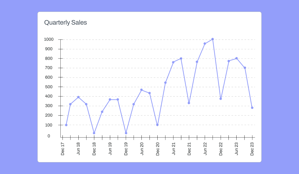
A sample of time series data reflecting quarterly sales | Source: Pecan AI
Naturally, we expect ice cream sales to be higher in the summer months and lower in the winter months, with spring and fall typically somewhere in between, perhaps depending on weather conditions.
The seasonal nature of the sales is essential to understanding and forecasting sales activity, and we need more than just a single distribution of values to capture the actual movement and variation in sales over time. The sequence of values is important, too.
Why do we need to identify abrupt change points for machine learning?
When that characteristic sequence of values in our data is suddenly thrown off, that alteration causes a significant change in the structural behavior of our data.
After all, machine learning models don’t like significant changes in data’s behavior. Their purpose is to learn patterns from data, and when those patterns are substantially disrupted all of a sudden, models can do strange things.
For example, a model that relies on something being constant, like the coefficients of variables in a linear regression model, can begin to suffer from Simpson’s Paradox.
What does that mean in practice? When looking at all the data together, the model may identify one particular pattern that seems most prominent. However, in reality, if the data were divided to reflect what occurred “before” and “after” a disruption, very different patterns would better represent the data.
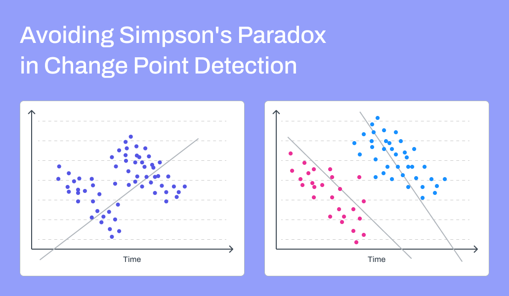
In this case, using all the data points as shown on the left would result in a model that would generate the single line shown, reflecting what looks like a positive relationship between the variables. But, as shown on the right, if the data were divided into two groups reflecting data points before and after a disruption, each group would be more accurately described with distinct models reflecting negative relationships — a totally different interpretation. | Source: Pecan AI
As I discussed in my recent blog post on estimating baseline for marketing mix modeling, we use state-space models at Pecan as part of our MMM procedure. However, even these models, which are time-variant (meaning they consider the passage of time and how it affects the predicted outcome), are thrown off by abrupt change points. The time variance is strongly affected around the change point. The model can become optimized to minimize errors around that point, a behavior also seen with other kinds of outliers. The model can be sensitive to features that aren’t very informative about much of the data but are highly correlated around the change point.
With all of these impacts, the interpretation of models can become highly spurious (i.e., misleading). Unfortunately, that’s especially true for econometric-style use cases like marketing mix modeling.
Why many approaches to abrupt change point detection don’t work
There are some traditional change point detection methods we could try:
- Bollinger Bands: This approach comes from technical analysis in finance. Essentially, we’d build a moving window that includes where we estimate the next data point will be, as well as an interval reflecting its high and low possible values based on standard deviations. Many variations on this approach exist, but they all share the same basic structure: an analysis of the distribution of the value being measured, such as a stock price or sales total, by focusing on a central value and its variability.
- Residual analysis: We could build a model that attempts to predict our outcome variable and then use that model’s accuracy to determine the likelihood of where the change will be. Wherever the model is “unusually wrong,” we might identify that as a potential outlier or a change point.
Bollinger Bands, while they do anticipate the expected direction of future values, are limited by the way they treat all data in the chosen window equally. Last week’s ice cream sales may be less relevant than last year’s sales as we transition from summer to autumn.
Residual analysis depends on training a model to accurately capture expectations, and there are a lot of challenges with this approach when the goal is change point detection.
For example, maybe your ice cream company introduced a Halloween-themed ice cream that shot sales through the roof one October. Q4 sales were suddenly much higher and even beat summer’s Q3 sales. Or maybe an unusually hot spring season meant sales were abnormally high as customers sought frosty treats earlier.
Additionally, if your overall sales trend is “up and to the right” simply due to consistent growth in demand, you’ll probably reach a point where, say, winter sales would be higher than the preceding spring’s sales.
How can we incorporate all of these potential shifts into an effective model? We could try a traditional time-series approach, but we’d end up with a vast range of options. With a common approach like exponential smoothing, we’d have to consider whether the data is seasonal, what the periodicity is, and so on. With dozens or even hundreds of models to consider, it’s pretty much impossible to know which is the “true” one.
But hey, we can automate things and have plenty of compute! Let’s just train all of those potential models and choose the best one. Sound good?
Unfortunately, that doesn’t work either. We still won’t be able to tell which model is best. Accuracy is difficult to assess because we’re looking for change points, and we expect periods where the model will be wrong due to those changes.
Let’s imagine we could build an effective model selection process. But then we add a little new data into the mix. Suddenly, our selection process identifies a different “best” model. With that new selection, we might reconsider whether a specific data point should be regarded as a change point.
One more scenario: Our model selection is somehow stable, and we actually do choose a model with the same configuration each time we test it. We would still face the issue that many traditional time-series forecasting models use simplistic assumptions, such as assuming that the trend is linear throughout the series and doesn’t vary (e.g., it never becomes a nonlinear trend). Your through-the-roof Halloween ice cream sales might represent a nonlinear growth moment, and the model wouldn’t be able to account for that.
How Pecan deals with abrupt change point detection
Despite these challenges, we’ve implemented an approach that contends with all those issues (do we get an ice cream reward?).
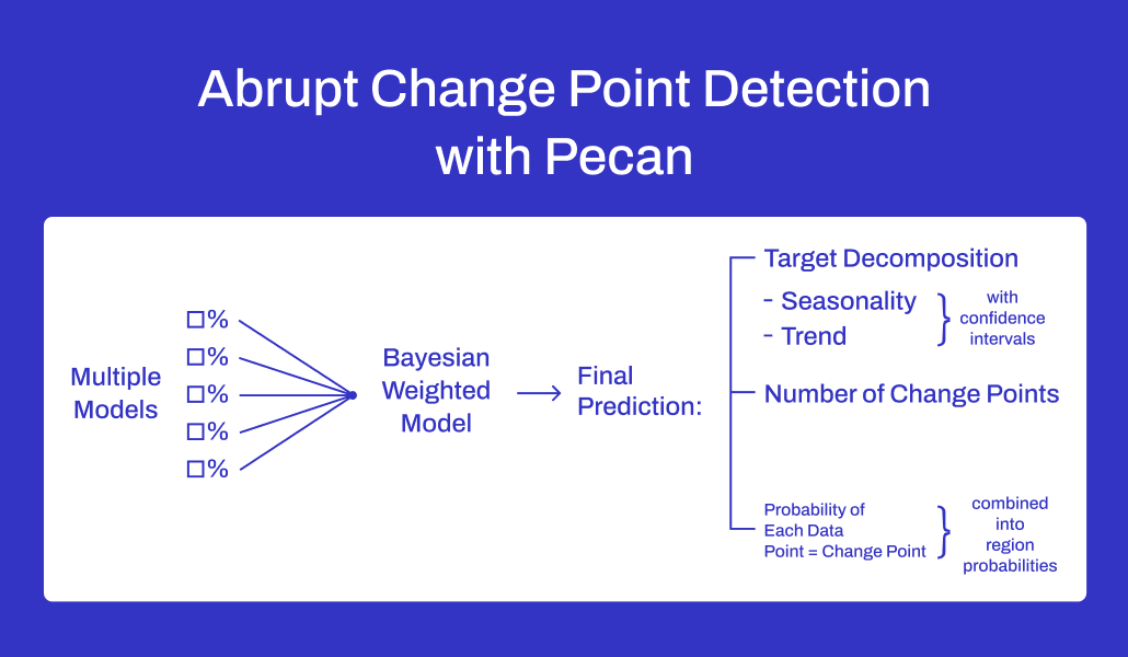
Two key elements distinguish our approach. First, we don’t use a traditional single best model selector to identify the right model for the situation. Instead, we create a Bayesian weighted model, which takes inputs from multiple weighted models and doesn’t settle on a single model structure or parameter to explain the target. Each model is given a probability that it reflects the true model, and each makes a weighted contribution to the final prediction.
Second, we incorporate a model component specific to abrupt change point detection. That component estimates two parameters: the number of change points and when the change points occur.
The first output we get in this approach is the decomposition of the target into two additive components — seasonality and trend — as well as a confidence interval for their true values. The second output is the number of change points. Because that number is a parameter generated by multiple models, we calculate a central value from all of them to use as the final value. And finally, the third output is the probability that each data point represents a change point.
When we process these outputs, the point probabilities are combined into region probabilities for further analysis. It might be the case that a change occurs over a few periods, and while each individual point isn’t that significant, the combined impact of multiple points is meaningful.
How Pecan addresses change point direction
Finally, we can use the number of change points — the second output mentioned above — to select the data points with the highest combined probabilities. These data points are those we then identify as change points for further evaluation.
How does identifying these change points change our MMM models?
With these points identified, we first can enrich our exploratory data analysis (EDA) with these data points. We might be able to identify singular events related to these change points to help determine which are important and which aren’t. Comparing these change points to other datasets might also help us determine what drove these unexpected changes.
Identifying these change points can also inform meaningful conversations with business stakeholders about their data and business. For example, in discussing notable change points with a customer recently, we learned that a change point coincided with competitor activity. That additional insight highlighted that we should include competitor information in the model.
In a predictive project, we might also consider using a training dataset that begins after a notable change point. As mentioned above, ML models don’t tend to do well when faced with data observed under different structures.
This careful selection of training data can be especially critical when we build a model that provides an output to be used as a feature in another model, as we do in our baseline estimation. A change point would result in needing to train two models: one on data before the change point and one on data after it. That approach would prevent the model from trying to smooth the transition between before and after the change, instead of treating it more appropriately as a structural break.
Ongoing innovation in marketing mix modeling
With efforts like this, Pecan continues to implement innovative MMM approaches to address today’s marketing challenges and help our customers achieve their goals.
If you’re looking for support in using MMM to make all your most important KPIs go “up and to the right,” we’re here to partner with you, for change point detection and beyond. We’d love to give you a guided tour.